What I learnt making Android games from scratch

There are two ways you can build something:

1, Build on top of an established system
2, Build from scratch

While building on top is an obvious practice for software that sells, It is when projects are build from scratch which gives you a deeper understanding.

I have spent the last 3 years on and off building games from scratch ( using canvas, media player, bitmaps, threads, classes etc) for Android and here are my experiences:

1, The seemingly easiest problems are the toughest one:

A lot of times, problems seem easy when you do not understand them properly. Building games involves coming across dozen of such cases on a regular basis where your assessment mismatches reality which is often disappointing. For me, this involved around 80% of issues dealing with threads. You see, when you see a sprite moving on screen independent of game environment, that animation is a thread. A lot of times I used to find myself back at the drawing table trying to add one more level of interaction between the sprite thread and the main game thread. 

So before you go ez-pz on a problem, ensure you are not pushing yourself into muddy waters.

2, The documents are never complete:

This covers everything including documentation for android, an audio library that you are using and surprisingly your very own project. When you are dealing with a lot of parallel ideas, just commenting the code is not enough. Having a running document while you are building the game is the most mundane yet the most efficient of decisions. Your future self or your peers will thank you for this.

3, Things on the internet disappear:

You must have come across the statement: "If it's on the internet, its there forever". Sounds good, but there's another side to it. The web is constantly changing. This means while a lot of content is coming into new existence, a fraction of it also snaps out of it never to be seen again. This largely involves mid-tier knowledge that ties low level details with high-level abstract implementations ( looking at you bitmaps). Documentation again can save the day by bundling this knowledge into the project.

Another example is volatility of 3rd party dependencies. Remember Parse by facebook? or TinyPic? No right? They shut down! So no matter what company is behind a service (It was facebook godamnit!), It can disappear. However staying updated with your inbox saves you the hassle of cases like LOOSING ALL DOCUMENTATION DIAGRAMS TO TINYPIC SHUTDOWN! You get the idea what I am implying here.

4, Don't fool yourself:

So your game is good right? You sure buddy? You know how all parents think their newborn is the cutest of all the newborns that have ever existed?!! ( I mean come on peeps! Clearly my future kid is the cutest!). 

The point is, just because you invested a lot of time into it, doesn't mean it will turn out great. (This is not about kids anymore, but who am I to judge?)

Being rationally critical of yourself is one of the first steps to building cool things ahead. So if your game sucks big time, Its time to toss it in the bin! ( or get into fixing it if you are that stubborn). 

Remember, you are in this to learn. Honouring critical feedback is one of those learnings. This brings us to the next point.

5, Honour Feedback:

You will be tempted to ask others to play your game and they might not like it. Don't let this get to your head and above all, never take it personally. I have experienced that giving critical review is one of the most caring acts. What blocks us from reaping the benefit is how we take it. Think for yourself: If you didn't care for the project, why would you tell me what is wrong with it? Thinking this way requires major perception shift, The benefits break major mental bounds for everything you do going ahead.

6, Enjoy the struggle!

No Seriously! Its a game after all right? And while you might not have an audience in sight for your project when you begin, you can always pivot to monetise! The struggle you did while building gets fulfilled by the joy when someone appreciates your work. A lot of top titles started out as side hobby projects and they were definitely not the author's first project.


------------------------------------------------------------------------------------------------
If you liked or disliked what you just read, let me know in the comments.

P.s.  I do coffee if you pay.

Follow me on Twitter here: @Sanjeev_309
Connect on LinkedIn here: LinkedIn

Read more →

What does a CNN see? : Visualising hidden layers of a Neural Network

Deep Learning has made remarkable progress over the past few years with quick transitions from discovery of new methods to their industrial implementation. While framework and libraries have made creating and working with deep architectures easy, quite less is known by practitioners about the internal states of the process. This post is an attempt to find out what composes a neural network and what a convolutional neural network sees in an input.

The code is publicly available on my Github

The architecture of the network we will work on is as follows:

Input
Convolution (5 x 5)
MaxPooling
Convolution  (5  x 5)
MaxPooling
FullyConnected

The model is trained on the popular MNIST dataset with following parameters:

batch_size = 50
learning_rate = 0.001
epochs = 400
Optimiser = Adam

After training, we load the layer to visualise and pass a sample input via the input layer. The function then runs a session for the layer given the input and returns all the filters that comprise that layer.
This is done by using TensorFlow's session.run() function which returns all the filters when a layer is fed in as an object.

Sample Input:

The results for the sample input are the following visualisations which are plot using matplotlib.

Hidden Layer 1 :

 Hidden Layer 2:

The number of plots correspond to the increased number of filters as we go deeper into the network.
The depth also describes how more finer details are sought by the filters as the depth increases. This can be seen in the representation between what HiddenLayer1 vs HiddenLayer2 sees as the filter shows how the input stimulates the filter.

The height of your accomplishments equal the depth of your convictions.

Stats:
TensorFlow 1.8
Jupyter notebook
Ubuntu 17.10

Read more →

What's that Noise? : Working with sound on Android

Sound is diverse. It's nature is to comprise of so many forms that solid rules cannot draw lines between them. I always have been an admirer of sound.

I have spent a few weeks implementing sound acquisition and processing in android and have come up with something to begin with.

Presenting:

Shh..Silence 

An application that monitors sound level of an environment and plays a 'Shhhh...' when noise levels pass a limit.

You can download it here:

Google Play and the Google Play logo are trademarks of Google LLC.

For the end user, it is a harmless application but from an engineering point of view, the internals are a window to a ton of possibilities. 

The application monitors sound in the following manner : 

1. Acquire Microphone 
2. Configure 
• Sample Rate
• Mono/Stereo
• Encoding format
• Buffer size
3. Calculate average over the buffer size
4. Compare obtained value with threshold 
5. Trigger when above threshold

The pipeline is simple when dealing only with the average. Here's a code snippet for step 3:

 private void readAudioBuffer() {  
     try {  
       short[] buffer = new short[bufferSize];  
       int bufferReadResult = 1;  
       if (audio != null) {  
         bufferReadResult = audio.read(buffer, 0, bufferSize);  //Audio Samples
         double sumLevel = 0;  
         for (int i = 0; i < bufferReadResult; i++) {  
           sumLevel += buffer[i];  
         }  
         lastLevel = Math.abs((sumLevel / bufferReadResult));  
       }  
     } catch (Exception e) {  
       e.printStackTrace();  
     }  
   }  

The most intriguing part of it is at bufferReadResult. It contains a sequence of numbers that depict the sound received by the microphone. Following this, it is a matter of requirement what needs to be done next. On extracting audio features like Mel Coefficients, MFCC etc, the application can be stretched to domains of Audio Classification, Speech Recognition, User Identification and Keyword Detection.

Implementing ML/DL on android has become easier than ever using TensorFlow with a light framework. The next step is to develop an application that uses TensorFlow for purpose of classifying sounds.

The Optimist sees the potential in a seed

Kudos.

Read more →

An Infinite point possibilities : Intel's Open3D Library

Intel have recently launched its open source library for 3D data processing Open3D  [ research paper by Qian-Yi Zhou and Jaesik Park and Vladlen Koltun ]

*not the official logo, only for personal representation

Open3D is an open-source library that supports rapid development of software that deals with 3D data. The Open3D frontend exposes a set of carefully selected data structures and algorithms in both C++ and Python. The backend is highly optimized and is set up for parallelization. Open3D was developed from a clean slate with a small and carefully considered set of dependencies. It can be set up on different platforms and compiled from source with minimal effort. The code is clean, consistently styled, and maintained via a clear code review mechanism. Open3D has been used in a number of published research projects and is actively deployed in the cloud.

With Open3D, the library enables developers to work with 3D models and point clouds.
Open3D has the following features:

• Basic 3D data structures
• Basic 3D data processing algorithms
• Scene reconstruction
• Surface alignment
• 3D visualization

With Open3D, RGBD images (Images with 3 color components and a Depth component) can be converted into 3D models. Here' a python code snippet to achieve just that:

 import sys  
 import py3d  
 import matplotlib.pyplot as plt  
 sys.path.append("../Open3D/build/lib/")  
 print("Read Redwood dataset")  
 color_raw = py3d.read_image("/home/<username>/Open3D/build/lib/TestData/RGBD/color/00000.jpg")  
 depth_raw = py3d.read_image("/home/<username>/Open3D/build/lib/TestData/RGBD/depth/00000.png")  
 rgbd_image = py3d.create_rgbd_image_from_color_and_depth(  
     color_raw, depth_raw);  
 print(rgbd_image)  
 plt.subplot(1, 2, 1)  
 plt.title('Redwood grayscale image')  
 plt.imshow(rgbd_image.color)  
 plt.subplot(1, 2, 2)  
 plt.title('Redwood depth image')  
 plt.imshow(rgbd_image.depth)  
 plt.show()  
 pcd = py3d.create_point_cloud_from_rgbd_image(rgbd_image,  
                        py3d.PinholeCameraIntrinsic.prime_sense_default)  
 pcd.transform([[1, 0, 0, 0], [0, -1, 0, 0], [0, 0, -1, 0], [0, 0, 0, 1]])  
 py3d.draw_geometries([pcd])  
 print("Writing ply file")  
 py3d.write_point_cloud("Redwood.ply", pcd)  

The result obtained is as follows:

Open3D has been developed keeping in mind the computations required for solving 3-dimensional geometry and the need for parallelization for faster turn-around times. It has an inbuilt visualiser which enables developers to visually examine their work and also manipulate them using pan and rotate controls along with a dozen more manipulations such as lighting, changing point size, toggling mesh wireframe etc.

Open Source community has always accelerated the development of advanced tools and libraries. Looking forward to the community to scale this one ahead too.

Limitations only exist if you let them

<This post is an attempt to integrate 3D model in a webpage using webVR, stay tuned for a post update>

Peace Out.

Read more →

Project AlphaUI : Computer Vision and Virtual Menu Navigation

We have always sought of new ways to interact with computers. From typed commands to automatic speech recognition, the aim is to make it appear natural to us, as if not interacting with a computer but a Human.

Project AlphaUI

AlphaUI is a virtual menu interface that lets you interact naturally with the GUI displayed. It works by using a webcam to capture live frames and through Image Processing finds out where the user wants to point out in the given space.

The Program is written in C++ using OpenCV 3.1.0 Library and performs the following operations on each image from which relevant information is extracted.

• HSV Segmentation
• Dilation
• Eroding
• Centroid Detection
• Calculation of Image Moments
• Alpha Blending

For the project to be demonstrated, I have utilised my computer vision project: Automatic Face Recognition System. The AlphaUI interface is built on top of the Face Recognition System with a custom GUI giving integrity to both projects.The functional response of interface have been disabled for the demo. Any developer can define their own GUI for their system that require user interaction in the same way.

Screenshots of the system: 

The AlphaUI interface

Ball tracked continuously by the system

Touchless Interaction with the interface

The system can be trained on any object of interest provided it is distinct in color (read HSV segmentation) . The training is done by repeatedly marking all over the object with the mouse pointer. This step has to be done only once in a lifetime or when you need to use a new marker. The values are saved in a text file to be reused in next run.

Disclaimer:

This project was done about an year ago but never saw daylight until now. What would you do with the possibilities of this project? Do comment and let me know.

Step By Step One Goes Very Far

Used:

Ubuntu 16.04

Code::Blocks IDE

OpenCV 3.1.0 : C++

Read more →

Visualising N-Body Simulation in OpenCV : Multicore Processing with OpenMP

The Good side of OpenMP is its inherent simplicity. The ease with which it enables you to write parallel code is remarkable.

This post is an update to a previous post: Building OpenCV with OpenMP . In this post, it's all about performance analysis of OpenCV with and without OpenMP.

The code being used is the popular N-body Simulation used to simulate gravitational effect on large particle systems. I have used source code as available on Mark Harris's github repo with a few modifications.

Modifications made are as follows:

• A 2-D Coordinate system in place of a 3-D system for visualisation in OpenCV
• Integer precision for co-ordinate calculation for visualisation.
• Integer time step dt which determines the speed of our simulation . 
• Drawing circles with radius = 0, giving us particles the size of a unit pixel.
• Dynamic Window size declaration and adaptation
• Re-Wrote random coordinate generation method for 2-D coordinate system.

The modified source code is available on my github profile/visualise-nbody-opencv  

Benchmarking: 

Approach #1: Total Execution Time
The Total Execution time for computing N iterations for the particle system is directly indicative of performance for N-body Sim. In general terms, if N iterations take time T on a single core , then N iterations should theoretically take time T/4 on a Quad-core CPU. Though this might not always be the case, it is a good parameter to evaluate.

Approach #2: CPU Resource Monitor
All OSes are bundled with a resource monitor that maps CPU utilisation with time.The resource monitor is an effective tool to visually examine the CPU per core usage.

A combination of approach #1 and #2 is used to examine OpenCV with and without OpenMP parallelization.

Have a look at what my code for N-body simulation for N= 2500 particles looks like:



The following benchmark has been evaluated for 1000 iterations of 2500 particles.

EVALUATION:

• Without OpenMP Parallelization

Time:
time is a command in the Unix operating systems. It is used to determine the duration of execution of a particular command.

  time ./nbody
  real        2m7.258s
  user        1m37.096s
  sys         0m0.500s  

CPU Core Usage:

The calculations being done on a single core with occasional core switching 

    The CPU usage graph shows that at any given time, Only a single core is being used for the calculation. Additionally, the core being used is also switched by the OS occasionally.

• With OpenMP Parallelization

Time:

   time ./nbody
   real        1m23.373s
   user        3m31.596s
   sys        0m0.696s 

CPU Core Usage:

The CPU usage during OpenMP being used is sufficient to show that the code is run parallel on multiple cores. The CPU time shows the same as we have a reduced real time (as in wall time) by running computations on 4 cores of the CPU. For details of how to interpret the time output, refer this answer on Stack Overflow.

OpenMP is therefore an easy to use framework in cases where code needs to be distributed on multiple cores. Since its inception, it has advanced sufficiently and have been adopted among developers looking to leverage improved hardware capabilities. 

To Know more about OpenMp, visit their official website.

Kudos.

Push Yourself Again and Again.Don't give an inch until the final buzzer sounds.

Stats:

Ubuntu 17.04

Intel(R) Core(TM) i5-4200U CPU @ 1.60GHz

8 GB DDR3 RAM

Code::Blocks 16.01

GCC 6.3.0

Read more →

Stepping up the game : Building OpenCV with OpenMP

OpenCV API has been a choice for Image Processing over MATLAB for quite a while now especially on an SoC like Raspberry Pi 3.

However I always had an inquisitive concern (too fancy?) whenever I ran an OpenCV project (as in my previous project for Real-Time Face Recognition System ) that when it seemed that the CPU is doing the best it can, the CPU usage graph never went above 25%.

Since Raspberry Pi has a Quad-Cored BCM 2837 , this meant that the program is using a single core for all the tasks. The fact that my applications are unable to exploit the resources that are available posed a problem to be solved; OpenMP to the rescue.

OpenMP API 

Why OpenMP :

Because it is simple and since Raspberry Pi has no significant GPU (for High Performance Computing) which puts OpenCL out of question and no Nvidia tag anywhere puts CUDA out of the picture too. OpenCL can be implemented on a CPU too but the lead time and the overhead will be too much for now.

OpenMP API is designed for multi-processor/core, shared memory machines and has a compiler directive based usage which though simpler to implement does require careful considerations. A thoughtless "#Parallel For" loop can significantly back fire and cause things to break.

A number of tutorials and documentations for OpenMP API are available.Two of those:  here and here!

Building OpenCV with OpenMP requires a simple addition at the building process:

 cmake -D CMAKE_BUILD_TYPE=RELEASE -D WITH_OPENMP=ON -D CMAKE_INSTALL_PREFIX=/usr/local ..  

I also used my tried and tested method of building extra modules that has never failed me since its discovery.
The building process starts and completes as it should with the following OpenMP tag somewhere in the entire log:

  Parallel framework:      OpenMP  

The OpenMP and OpenCV seem like a good pair to work with on Raspberry Pi.
Will post an update to my inquisitive concern after I get the OpenMP implementation done.
Lot of directives to add.

Update [27/Aug/17]: Added follow up post : Multicore Processing using OpenMP

There are no wrong turnings. Only paths we had not known we were meant to walk.

Peace Out.

Stats:
Ubuntu 16.04
OpenCV 3.2.0
GCC 5.4.0

Read more →

Automatic Attendance System using Face Recognition ( OpenCV 3.1.0 & Raspberry Pi )

Project Phase

A Face Recognition system to be used for marking attendance in an organisation for a streamlined and centralized record of Employees or Members.

Phase includes the following stages:

• A C++ program to detect and store faces. (Detection)
• A Python Script to maintain and link available faces. (Linking)
• A C++ program to fetch faces from a camera and compare them with available database. (Recognition)
• A Python Script to update the record on Google Spreadsheets over a secure wireless connection. (Uploading)

All of this runs on a Raspberry Pi 3.

Phase is and has been my most ambitious project because of the way it works. And also because it is composed of three of my most relished domains: Embedded Linux, Machine Learning and Internet of Things.

Each Functional component took considerable time worth mentioning in this catalog however I also do acknowledge that a lot of hows and whys will still be skipped because they are really large in number.
Last but most important, Kudos to Stack Overflow and every developer that asked relevant questions for this project of mine to be completed even after so many dead ends I have encountered.

Project Phase:

My initial setup was Ubuntu 15.10 on an Intel core i5 laptop. Linux was a choice because I already planned to deploy the final project on a Raspberry Pi. This maintained familiarity with the development platform.

The entire project is too long to discuss every working bit in a single blog post so an extended summary is what this post is.

What Phase Does:

It Sees You, Remembers You, Recognizes You and Keeps a note of it on Google Drive !
Pretty Cool when you think about it.
Each task stated above uses a separate program linked together to work seamlessly.

It Sees You:

The Video is captured via the integrated webcam (when developing on ubuntu) and via a USB webcam (when run on Raspbian OS [Raspberry Pi]).This is made easy by always fetching the video from the default connected device.As Pi doesn't come with an inbuilt camera,default device is the USB webcam.Voila!

A C++ program linked with the OpenCV (build from source:make,make install) running a cascade Haar's Frontal Face classifier detects the faces in an image.The task of detection is the following two things:

• Number of faces in the image
• Segmenting ,Cropping and Resizing Faces

Detecting One Face and Saving to Database

Detecting One Face and Saving to Database

A Video Documenting the database creation is as shown:

It Remembers You:

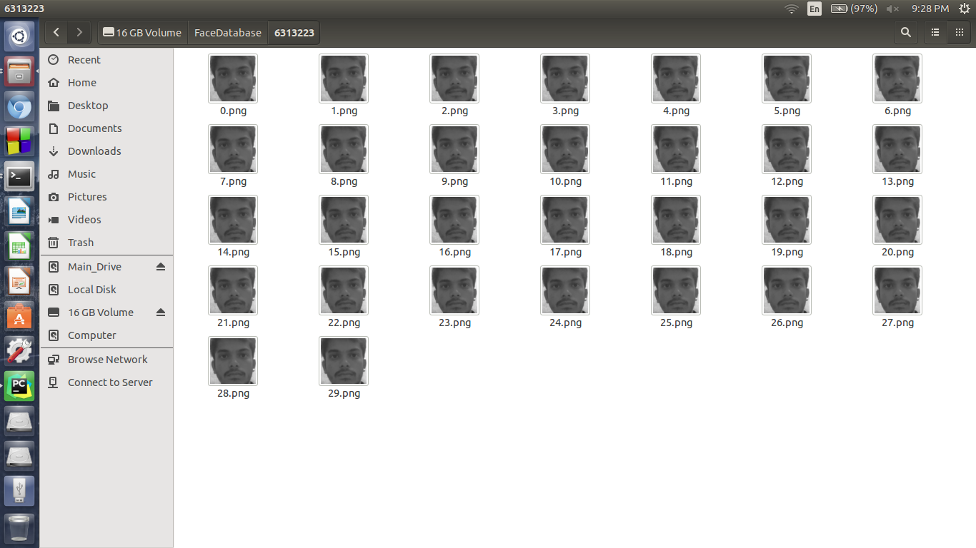
The database of a face is created only when only a single face is detected by the classifier.This ensures that the database of a single individual contains images only of that individual.Before saving the faces are gray scaled and resized to 300 x 300 pixels.

The structure of the folder is as :

.
|-- s1
|   |-- 1.pgm
|   |-- ...
|   |-- 29.pgm
|-- s2
|   |-- 1.pgm
|   |-- ...
|   |-- 29.pgm
...
|-- s40
|   |-- 1.pgm
|   |-- ...
|   |-- 29.pgm

A lot of guidance was received from OpenCV documentation.This includes the above folder structures to store faces.

Root Folder

Database of an Individual

Although the database of images is created successfully,For a program to actually "See" them,It is crucial that every image is properly documented along with the ID of the person they represent.This path creation and Labeling is done by a Python Script.

The Python script creates a record in .csv format which contains :

• Full Path of the image
• Label Corresponding to the Image

Since images are stored in a folder named after the id of the person, The name of the folder is infact the Label for our task.

The .csv file created looks like: 

/media/sanjeev309/28B8-7686/FaceDatabase/6313223/19.png;6313223 /media/sanjeev309/28B8-7686/FaceDatabase/6313223/18.png;6313223 /media/sanjeev309/28B8-7686/FaceDatabase/6313223/17.png;6313223 /media/sanjeev309/28B8-7686/FaceDatabase/6313223/16.png;6313223 /media/sanjeev309/28B8-7686/FaceDatabase/6313223/15.png;6313223 /media/sanjeev309/28B8-7686/FaceDatabase/6313223/14.png;6313223 /media/sanjeev309/28B8-7686/FaceDatabase/6313223/13.png;6313223 /media/sanjeev309/28B8-7686/FaceDatabase/6313223/12.png;6313223 /media/sanjeev309/28B8-7686/FaceDatabase/6313223/11.png;6313223 /media/sanjeev309/28B8-7686/FaceDatabase/6313223/10.png;6313223 /media/sanjeev309/28B8-7686/FaceDatabase/6313223/9.png;6313223 /media/sanjeev309/28B8-7686/FaceDatabase/6313223/8.png;6313223 /media/sanjeev309/28B8-7686/FaceDatabase/6313223/7.png;6313223 /media/sanjeev309/28B8-7686/FaceDatabase/6313223/6.png;6313223 /media/sanjeev309/28B8-7686/FaceDatabase/6313223/5.png;6313223 /media/sanjeev309/28B8-7686/FaceDatabase/6313223/4.png;6313223 /media/sanjeev309/28B8-7686/FaceDatabase/6313223/3.png;6313223 /media/sanjeev309/28B8-7686/FaceDatabase/6313223/2.png;6313223 /media/sanjeev309/28B8-7686/FaceDatabase/6313223/1.png;6313223 /media/sanjeev309/28B8-7686/FaceDatabase/6313223/0.png;6313223 /media/sanjeev309/28B8-7686/FaceDatabase/6313751/19.png;6313751 /media/sanjeev309/28B8-7686/FaceDatabase/6313751/18.png;6313751 /media/sanjeev309/28B8-7686/FaceDatabase/6313751/17.png;6313751 /media/sanjeev309/28B8-7686/FaceDatabase/6313751/16.png;6313751 /media/sanjeev309/28B8-7686/FaceDatabase/6313751/15.png;6313751 /media/sanjeev309/28B8-7686/FaceDatabase/6313751/14.png;6313751 /media/sanjeev309/28B8-7686/FaceDatabase/6313751/13.png;6313751 /media/sanjeev309/28B8-7686/FaceDatabase/6313751/12.png;6313751 /media/sanjeev309/28B8-7686/FaceDatabase/6313751/11.png;6313751 /media/sanjeev309/28B8-7686/FaceDatabase/6313751/10.png;6313751 /media/sanjeev309/28B8-7686/FaceDatabase/6313751/9.png;6313751 /media/sanjeev309/28B8-7686/FaceDatabase/6313751/8.png;6313751 /media/sanjeev309/28B8-7686/FaceDatabase/6313751/7.png;6313751 /media/sanjeev309/28B8-7686/FaceDatabase/6313751/6.png;6313751 /media/sanjeev309/28B8-7686/FaceDatabase/6313751/5.png;6313751 /media/sanjeev309/28B8-7686/FaceDatabase/6313751/4.png;6313751 /media/sanjeev309/28B8-7686/FaceDatabase/6313751/3.png;6313751 /media/sanjeev309/28B8-7686/FaceDatabase/6313751/2.png;6313751 /media/sanjeev309/28B8-7686/FaceDatabase/6313751/1.png;6313751 /media/sanjeev309/28B8-7686/FaceDatabase/6313751/0.png;6313751 /media/sanjeev309/28B8-7686/FaceDatabase/6313204/19.png;6313204 /media/sanjeev309/28B8-7686/FaceDatabase/6313204/18.png;6313204 /media/sanjeev309/28B8-7686/FaceDatabase/6313204/17.png;6313204 /media/sanjeev309/28B8-7686/FaceDatabase/6313204/16.png;6313204 /media/sanjeev309/28B8-7686/FaceDatabase/6313204/15.png;6313204 /media/sanjeev309/28B8-7686/FaceDatabase/6313204/14.png;6313204 /media/sanjeev309/28B8-7686/FaceDatabase/6313204/13.png;6313204 /media/sanjeev309/28B8-7686/FaceDatabase/6313204/12.png;6313204 /media/sanjeev309/28B8-7686/FaceDatabase/6313204/11.png;6313204 /media/sanjeev309/28B8-7686/FaceDatabase/6313204/10.png;6313204 /media/sanjeev309/28B8-7686/FaceDatabase/6313204/9.png;6313204 /media/sanjeev309/28B8-7686/FaceDatabase/6313204/8.png;6313204 /media/sanjeev309/28B8-7686/FaceDatabase/6313204/7.png;6313204 /media/sanjeev309/28B8-7686/FaceDatabase/6313204/6.png;6313204 /media/sanjeev309/28B8-7686/FaceDatabase/6313204/5.png;6313204 /media/sanjeev309/28B8-7686/FaceDatabase/6313204/4.png;6313204 /media/sanjeev309/28B8-7686/FaceDatabase/6313204/3.png;6313204 /media/sanjeev309/28B8-7686/FaceDatabase/6313204/2.png;6313204 /media/sanjeev309/28B8-7686/FaceDatabase/6313204/1.png;6313204 /media/sanjeev309/28B8-7686/FaceDatabase/6313204/0.png;6313204 /media/sanjeev309/28B8-7686/FaceDatabase/6313207/19.png;6313207 /media/sanjeev309/28B8-7686/FaceDatabase/6313207/18.png;6313207 /media/sanjeev309/28B8-7686/FaceDatabase/6313207/17.png;6313207 /media/sanjeev309/28B8-7686/FaceDatabase/6313207/16.png;6313207 /media/sanjeev309/28B8-7686/FaceDatabase/6313207/15.png;6313207 /media/sanjeev309/28B8-7686/FaceDatabase/6313207/14.png;6313207 /media/sanjeev309/28B8-7686/FaceDatabase/6313207/13.png;6313207 /media/sanjeev309/28B8-7686/FaceDatabase/6313207/12.png;6313207 /media/sanjeev309/28B8-7686/FaceDatabase/6313207/11.png;6313207 /media/sanjeev309/28B8-7686/FaceDatabase/6313207/10.png;6313207 /media/sanjeev309/28B8-7686/FaceDatabase/6313207/9.png;6313207 /media/sanjeev309/28B8-7686/FaceDatabase/6313207/8.png;6313207 /media/sanjeev309/28B8-7686/FaceDatabase/6313207/7.png;6313207 /media/sanjeev309/28B8-7686/FaceDatabase/6313207/6.png;6313207 /media/sanjeev309/28B8-7686/FaceDatabase/6313207/5.png;6313207 /media/sanjeev309/28B8-7686/FaceDatabase/6313207/4.png;6313207 /media/sanjeev309/28B8-7686/FaceDatabase/6313207/3.png;6313207 /media/sanjeev309/28B8-7686/FaceDatabase/6313207/2.png;6313207 /media/sanjeev309/28B8-7686/FaceDatabase/6313207/1.png;6313207 /media/sanjeev309/28B8-7686/FaceDatabase/6313207/0.png;6313207

The .CSV file created is used by the next segment to fetch,load and train the Face Recognizer algorithm.

It Recognizes You

The Task of Face Recognition is done by C++ Program written using OpenCV library.
The Face Recognition module is not native to the official source yet so the additional libraries are built using a new method I came up with as documented here.This method is more reliable than the conventional route.

The program fetches live feed from the default imaging device and processes it frame by frame.

The first task that the program performs is to train its Two classifiers on the training database and labels of images.The Two algorithms used are:

• Eigenface Algorithm   ( Principal Component Analysis)
• Fisher Face Algorithm ( Linear Discriminant Analysis )

Eigenface is single class specific i.e. It finds the similarities between multiple images of same individual whereas FisherFace finds the differences between different individuals.The Collective and commonly agreed result of both these algorithms trained on the same set of images is used as a confirmation of a prediction.

The Haar's cascade is run to segment the faces which are the evaluated by the two algorithms and predictions are returned by both.The value of prediction is accurate 90% of the trials however it depends on the quality of images in the database.

Video Documenting Face Recognition:

Keeping a note on Google Drive:

The task of connecting securely to google cloud is done by a python script. It uses the following package to do the task of accessing and updating attendance on google spreadsheet.

• Oauth2client  (Google Cloud Authentication Client)
• Gspread   (Google Spreadsheet API client)
• PyOpenSSL (Python Open SSL package)

The Result of prediction (Roll No. or Unique ID) is given to the Cloud Connect Script as a command line argument. The script fetches the date of current day from the system.These two data elements are enough to mark a student as present.

The Logic here is always a tautology, 

i.e. if a student 'A' arrives before the system ,he is marked as present for the current day.

      if a student 'A' is absent, he never arrives for attendance before the system, hence he is not marked for that day thus stating him absent.

The Python Script connects to a google spreadsheet via valid security credentials and update the attendance onto it.The programming is done in such a way that it handles all the possible scenarios that can arise on the spreadsheet section. Few of the problem -> solution are:

• Date Row not found -> Create row for Current Date. (When taking attendance on a new day)
• Roll No not found -> Create column for Roll No. (When database is updated)
• Date Row found, Roll No column not found -> Add Roll No column and write "Present" in current date row   (Database updated during current day)
• Date Row not found, Roll No. Column Found -> Add Date Row and write "Present" in current Roll No. column  (Database Intact, Day changed )

The Data for the recognized individual is successfully updated in 3-4 seconds. This is slow compared to execution time of our Recognizer program however keeping in mind all the authorizations and Credential check every time, it for sure is a lead over other unsecured connections.

The Google spreadsheet is edited to give write access to our API token so that there is no conflict of permissions during write task. 

Here is the video of Phase updating the attendance of a detected individual in real time:

The Pi Setup:

The Setup is done with a Dell VGA monitor using an HDMI to VGA converter to connect to Raspberry Pi. Additionally USB Webcam,Keyboard & Mouse are connected via USB port.The webcam lights are kept off because of high current surge of 6 LEDs. They barely make any improvements in lighting conditions anyway.

• An 8GB Sandisk MicroSD card is loaded with NOOBS and Raspbian OS is installed.
• OpenCV is built from source using my method for extra modules building as stated here.
• CodeBlocks is installed from apt-get and code is copied to from the ubuntu system to Pi using a thumb drive.
• Static path for database storage, database linking,fetching and cloud uploading are set to get around using command line arguments every time.The Detection stage still employs CL arguments to denote the person being databased.

The entire system is enclosed in a box as follows :

The LCD and the glowing Leds are part of a temperature monitoring system. It measures the temperature of the box internals to warn or ward off any heat damage. And that is an entirely different story for a later time.

-----------------------------------------------------------------------------------------------------------------
[ Update 17 November,2018 ] :

The code for a dlib variant of the face detection and recognition project is available for access on my github here : https://github.com/sanjeev309/face-recognition-dlib-tensorflow-knn
You will need to modify the core code to suit your requirement for an attendance system.
Pull requests are welcome.
-----------------------------------------------------------------------------------------------------------------


Success is not final, failure is not fatal: it is the courage to continue that counts

Used :
Code::Blocks IDE
PyCharm IDE
Raspbian OS
Atmel Studio 7.0

Read more →

ThinAVR v0.9: The Slim and Minimalist AVR development Board

A While ago I mentioned the need for a minimalist and cheap embedded development board .You may read my previous post here: Developing Slimmer AVR board

It was that day when I designed the prototype and today, I present to you :

A minimum AVR development board with what you need to get started.

The Initial Silk-less Give-Away model

Smooth Edges and Simplified design

Dimensions as that of a Credit Card!

Ergonomic and Simplified PCB Layout

The Size equivalent to the size of your credit card and powered by an ATmega32 at its heart .It gives ThinAVR the following capabilities:

In addition to the above features that are provided by ATmega32 alone, ThinAVR also comes with:

• A 16X2 LCD connection port mainly for program debugging operations,connected on Port C
• Additional Power and Ground Pins for interfacing external circuits
• External Crystal Oscillator for reliable UART/USART operations.The Internal clock just doesn't make it for UART
• Mounting holes on all 4 corners for a robust design
• In-Built ISP Port so that you can always reprogram your board.
• Push Button Power Switch because Reliability
• On Board Voltage Regulation for protection from over-voltages
• Power On Indication LED
• Ergonomic Dimensions the size of a credit card
• Sleek Look and Slim design

The board is expected to bridge the gap between a development board and a functional embedded system project by making the platform so affordable that each project has its own ThinAVR.

The Initial batch of ThinAVR has been distributed to aspiring embedded developers for a faster growth curve, proper feedback and a higher adoption rate.

ThinAVR v0.9beta :
-No Silk, Markings with a sharpie
-Female connectors for ports,Male Connector for 16x2 LCD
-12MHz Crystal Oscillator
-Embedded ATmega32
-Power Circuit
-Need ISP Programmer to burn programs.

The Next version therefore will have more or less things.

The Mightiest Tree grew from a tiny seed.

Peace Out.

Read more →

Line Follower using Neural Nets : Part 2 (Designing the Neural Net )

This post is the second in the series of developing a neural net line follower. For the post covering dataset generation, go here

Once data is handy, the next objective in a Neural Net is to plan out its structure.

Neural nets are mostly used for uncertain and non-linear operations as is our task of pattern matching a.k.a Classification.

A neural net has mainly the following layers which map the input to the output

• Input Layer
• Hidden Layer(s)
• Output Layer

The Number of Hidden Layer is a deterministic on the complexity of the task being performed.For example, A deep learning net might contain more hidden layers for a deeper defragmentation of data.However there is a trade off between Depth and Speed of execution, therefore for our case, a single hidden layer would be enough.

The Designed Network looks as depicted here:

8 : 1 mapping through a hidden layer of two nodes (and one bias unit)

Intuition says this will be sufficient for our task as a partition in half can easily tell which side of our sensor strip sees the line.

For details of what a neural network is, I would recommend going through the following site: Neural Networks and Deep Learning

For activation function in our network, I have used tangent sigmoid function:

Tangent Sigmoid Function

For faster development time, the neural net designer tool in MATLAB is used.For the sake of understanding, an algorithmic view is as shown:

x = 1 X 8;                                             {Input from 8 nodes}
W₁₂   =   2 X 8;                                     {Weight Matrix from Input layer to Hidden Layer}
Z₁= x*(W₁₂)^T = (1X8 * 8X2)= 1X2;   {Mapping from Input layer to Hidden layer}
A₁= TanSig(Z₁)= 1X2;                         {Activation of Hidden Layer}
W₂₃ = 1 X 2;                                        {Weight Matrix from Hidden layer to Output Layer}
Z₂ =A₁*(W₂₃)^T = (1X2 * 2X1)=1X1; {Mapping from Hidden layer to Output Layer}
A₂=TanSig(Z₂);                                    {Activation of Output Node}
Y=A_2;                                                                    {Output}

The specifications are set up in the NNFit tool in MATLAB and data obtained from the previous post is used to train the network using Backpropagation Algorithm. After the training completes, the entire process is stored as a script using the prompt window.

By default the script generated contains a lot of redundant information which can be optimised on examination.
The entire script is reduced to the following:

 function [y1] = NNLF(x1)   
 %NNLF neural network simulation function.  
 %  
 % Generated by Neural Network Toolbox function genFunction, 13-Aug-2016 14:40:30.  
 %  
 % [y1] = NNLF(x1) takes these arguments:  
 %  x = Qx8 matrix, input #1  
 % and returns:  
 %  y = Qx1 matrix, output #1  
 % where Q is the number of samples.  
 %#ok<*RPMT0>  
 %(c)Sanjeev Tripathi ( AlphaDataOne.blogspot.in )   
 % ===== NEURAL NETWORK CONSTANTS =====  
 % Layer 1  
 b1 = [-8.8516132798193108e-10;2.1615423176361062];  
 IW1_1 = [-30.312171052276302 -15.230142543653209 -7.5989117276441904 -3.8426480381828529 3.8426480396510354 7.5989117277872076 15.230142543113857 30.312171051352024;1.1787493338995503 1.1684723902794487 -0.30187584946551604 -1.2505266965306716 -0.85655951742083458 -0.61361689937359887 -0.51938433720151178 0.43601182390986715];  
 % Layer 2  
 b2 = -3.5519126834821509e-10;  
 LW2_1 = [1.0000000099939996 2.6043564908190074e-09];  
 % ===== SIMULATION ========  
 Q = size(x1,1); % samples  
 x1 = x1';  
 xp1=2*x1 -1;  
 xp1=cast(xp1,'double');  
 a1 = tansig_apply(b1 + IW1_1*xp1);  
 a2 = repmat(b2,1,Q) + LW2_1*a1;  
 y1=a2;      
 end  
 % Sigmoid Symmetric Transfer Function  
 function a = tansig_apply(n,~)  
 a = 2 ./ (1 + exp(-2*n)) - 1;  
 end  

The Neural Net being run uses the pre optimized weights to map the input to the output with an accuracy of 100% (High Variance) as the dataset contained all the possibilities. A demo of our net for different inputs entered manually is as shown:

As stated earlier,
        -1 informs to move left 
        +1 informs to move right 
        ~0 informs to keep moving forward

The network of nodes can compute with accuracy any width,orientation or order of line with absolute accuracy. It can also detect multiple lines simultaneously as the network has been trained for all the possible inputs that it can encounter.

An Implementation on AVR Atmega32 microcontroller to be covered soon.
Stay Tuned for more.

Peace Out

Used:
Matlab 2016a

Read more →

Line Follower using Neural Nets : Part 1 (Generating Data Set)

Neural Networks are convenient when mapping a function which behaves non-linearly. However, for Training and Testing purpose , Data is the most important piece of the puzzle.

The Neural Network Line Follower to be designed uses 8 Line sensing elements where each will return
 1 : Line Detected
 0 : Line Not Detected

So the possible dataset is the combination of 8 binary units arranged in different pattern leading to a total of
            2⁸ =  256 Samples of data.

I wrote the following MATLAB script to create the data for training the Neural Network.

 function [bin,out]=DataGen(m)  

 % Function to Generate Training Data set for training neural network of a  
 % line follower  
 %    
 %     [bin,out]=DataGen(number of inputs)  
 %       
 % It is a good practice to have an even number of input units for the  
 % NN Network to be trained  
 n=(2^m)-1;              
 bin=decimalToBinaryVector(0:n);   
 [p,q]=size(bin);             
 out=zeros(p,1);   
 bLeft=bin(:,1:(q/2));  
 bRight=bin(:,((q/2)+1):end);  
 wL=bi2de(bLeft,'left-msb');  
 wR=bi2de(bRight,'right-msb');  
  for i=1:p  
    if wL(i)>wR(i)  
      out(i)=-1;  
    end   
    if wL(i)<wR(i)  
      out(i)=1;  
    end  
    if wL(i)==wR(i)  
      out(i)=0;  
    end    
  end  
 end  

Here:
         bin holds the binary input sequence of 8 bits    
         out holds the output corresponding to the input bin

Such that:
          if bin=[1 0 0 0 0 0 0 0]  then out = -1      (Line Sensed on far left : Move Left)

          if bin=[0 0 0 0 0 0 1 0]  then out =  1      (Line sensed on right : Move Right)

          if bin=[0 0 1 0 0 1 0 0]  then out =  0      (Line sensed symetrically : Keep Moving Forward)

For a Neural Network,  0 is pretty much a perfection so it allocates a really small value (~0) such that it can be considered as zero.

From the script above with 8 as a parameter via the following syntax:

           [bin,out]=DataGen(8);

we get:

           bin = 256 X 8 Input Data Matrix

           out = 256 X 1 Output Data Matrix

In the screenshot of the varibles, Left Segment shows the input from the sensors while we have the expected output in the blue bounded box on right:

These Data elements are ready to be used as Training Parameters for our Neural Network.
Further Development to be covered by subsequent posts.

Update 7/Sep/16 : Read Part II: Designing Neural Network

Peace Out.

Used:
Matlab 2016a

Read more →

RoboAuto : Arduino Bluetooth Joystick for Android™

HC-05 has an added advantage in embedded systems that pretty much every smartphone is equipped with in built Bluetooth hardware.This opens up a large number of possibilities for access and control of embedded systems.

There are apps that do the task of controlling a system via bluetooth however none sufficed to my requirement. So I developed one,

Presenting  

RoboAuto

An Android Application for communication with HC-05 Bluetooth Module.
RoboAuto is a clean and effective app using which you can control your Robots or Devices with a Simple Joystick!
  

What RoboAuto does:

Program Flow

So, You as an embedded developer have to configure your robot only for the commands received from the app!

Here are few screenshots:

RoboAuto connects to the Bluetooth Module using a Wireless Serial Link. Android already provides support for this in their native API.

After a successful connection, characters are sent to the module on actuation of joystick ,buttons or check boxes which can be read and executed by Arduino™ or other microcontrollers.

Special Thanks to zerokol for his JoystickView Library.
The Joystick sends the following :

Forward: F
Backward: B
Left : L
Right : R

Additionally I have assigned intermediate directions , for example, FL for Front-Left, BR for Backward-Right and so on.
No Changes are to be required on the Embedded side as the UART only parses a single character at a time, giving us simultaneous (in theory) Forward and Left motion. Kind of like what happens in a PWM.

Download RoboAuto here:

Google Play and the Google Play logo are trademarks of Google LLC.

This Post therefore will be updated soon and is worth a bookmark.
UPDATE (22/October/17): Savvy has been renamed to RoboAuto and published on Google Playstore
UPDATE (10/August/16) : Few Screenshots and content have been updated!
UPDATE (25/August/16 ):  Savvy(Now RoboAuto) is available for testing and debugging for FREE
UPDATE (12/September/16): Added Internet Access permission for Google Form Integration.
UPDATE (19/March/17): Fixed a lot of bugs in the layout scale. Renamed "Turn Light" to "Rear Light."

Do report any bugs you encounter.
Credits (19/March/17):  Thank You Shivani for your Feedback on Design Issues

Good Stuff Take Time.

Used:
Android Studio 2.3.3
Lenovo S6600 , Micromax Knight Cameo for Debugging.

Read more →

Programming and Simulation of AVR with HC-05: PART II

The final build of my work with HC-05 involves using AVR ATmega32 microcontroller which is a powerful micro controller. The Controller is programmed in AVR GCC.

For HC-05 (or any other serial communication system), the USART needs to be set on the ATmega32 through programming.
Here is a snippet of code being used for UART in my build:

Setting up UART

The Primary task of responding to various commands is done by a switch statement which is way easier to modify and work on instead of  IF-ELSE statements.Since Each character has a unique ASCII Code, we have a lot of commands which can be given to the micro controller.For example ,there are 26 lower case + 26 upper case + 10 digits + about 32 symbols which equal about 94 unique commands.
Snippet of code for Switch:

Decision Task by Switch Statement

The character 'ch' is set to receive value from registers whenever the receive interrupt is triggered by the HC-05.The ISR (Interrupt Service Routine) is defined as follows:

Interrupt Service Routine

Simulation of code is done in Proteus 8.4 using all the peripherals included. Input here is given from a virtual terminal however HC-05 would have served the same objective.

Simulation in Proteus

A video accompanying the simulation conveys that the code works fine and can be implemented into the hardware.Here's the vid :

Used:
Proteus 8.4
Atmel Studio 7.0

Read more →